Measuring Energy Savings

Home Energy Audit Homework: Solutions

Prof. Richard Sweeney

Economics of Energy and the Environment
Econ 3391.01
Boston College

2026-10-22

Recap from last lecture

  • We have some idea about the benefits of a policy?
    • ie McKinsey analysts did some calculations for energy efficiency
    • Other contexts: returns to college; impact of health insurance on health outcomes; impact of free daycare on women’s workforce participation
  • But we know that this is complicated
    • Homes / people are different
    • Real world outcomes depend on many factors
  • We want to use real world data to estimate the benefits of policy
    • Can be used for cost-benefit analaysis/ optimal policy design

Measuring real world policy benefits is challenging for two reasons

  1. The effect varies across people
    • Some homes are old and inefficient, others are new and efficient, etc
  2. People select into the thing we want to measure
    • In order to estimate the effect of energy efficiency, we need some people to get the efficient good and some not to
    • If this choice is intentional, the outcomes will vary across people who do and don’t get it.
  • This problem set illustrates these issues with a specific (made-up) dataset where we know the true answer.
    • Given that, we can compare what we get using econometrics to the truth

Overview

Topic: How do we measure the benefits of energy efficiency policies?

Key Concepts (from lecture):

  • We only ever see one potential outcome for each household: \(Y_{i1}\) or \(Y_{i0}\)
  • Getting an audit is a “purposeful” decision, so audited and non-audited households differ
  • Different comparisons yield different answers. Some have a causal interpretation, others do not.

Methods Covered:

  1. Average Treatment Effect (ATE)
  2. Voluntary Opt-in & Selection
  3. Naive Comparison & Selection Bias
  4. Randomized Experiments
  5. Random Encouragement: Free Audits
  6. Intent-to-Treat (ITT)
  7. Local Average Treatment Effect (LATE)

Background

Home Energy Audits

What is a home energy audit? (e.g., a Mass Save Home Energy Assessment)

  • Energy specialist visits your home
  • Inspects insulation, windows, heating and cooling systems
  • Produces a report of recommended upgrades, with predicted savings for each
  • In Massachusetts: the gateway to subsidized insulation, heat pumps, etc.

Policy Goal: Reduce information barriers to energy efficiency adoption

This homework: Unlike Mass Save, audits cost $250, and a household decides whether to get one.

A Unique Dataset

We have an unusual dataset with parallel universe observations:

Variables:

  • y10: Spending WITHOUT audit (\(Y_{i0}\))
  • y11: Spending WITH audit (\(Y_{i1}\))
  • ey10, ey11: Expected spending
  • hassle: Audit hassle cost (\(\xi\) from lecture)
  • (y00: Pre-period spending, unused)

Example: Household 1

  • Expected without audit: $1,843
  • Expected with audit: $1,486
  • Actual without audit: $1,874
  • Actual with audit: $1,548
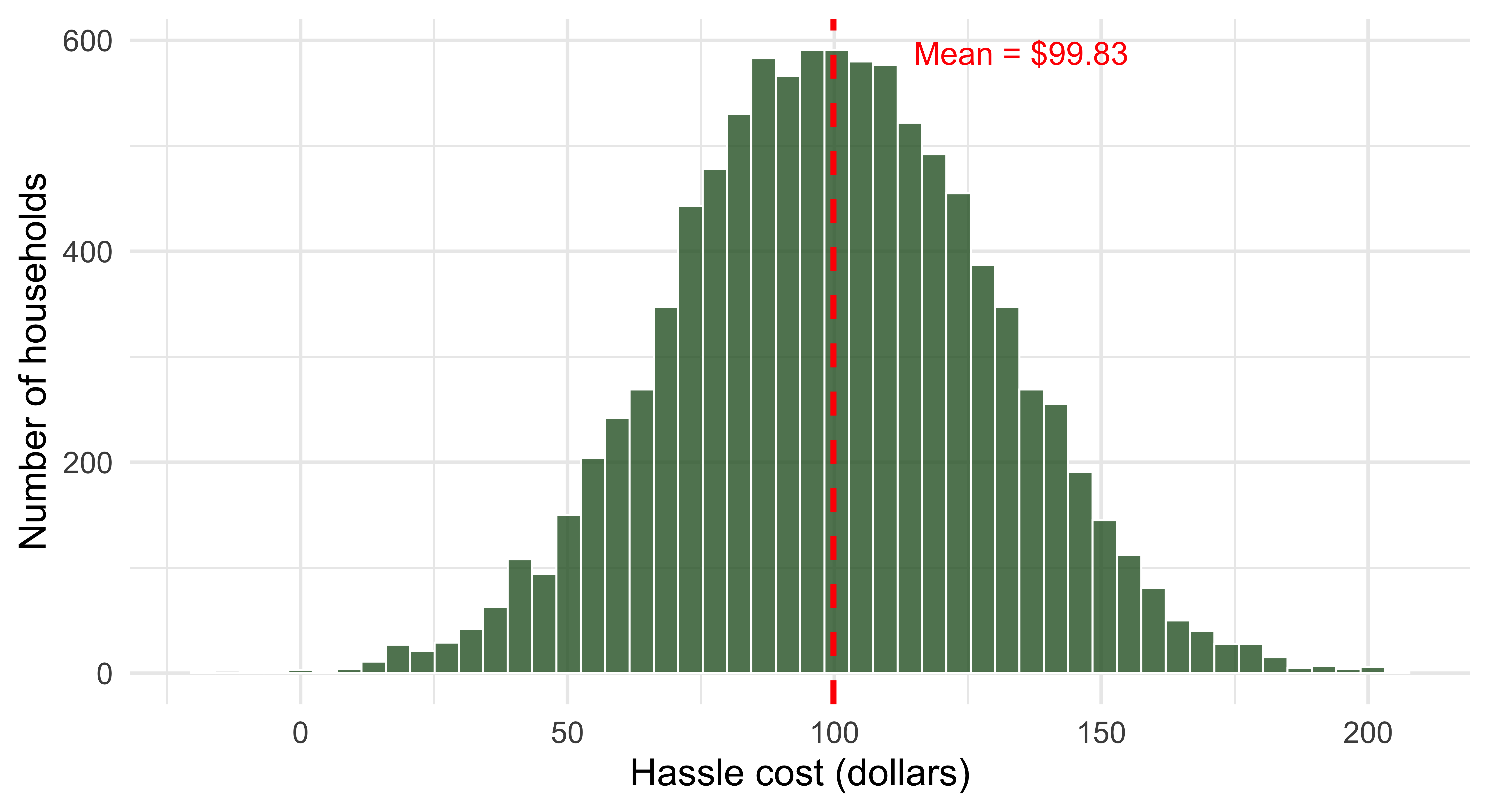
  • Hassle cost: $99.83

Key Point: We observe both potential outcomes for each household!

Challenge: In the real world, we never have parallel universe data!

Only observe:

  • y10 if household didn’t get audit
  • y11 if household did get audit
  • NOT hassle costs or expectations

This is the Fundamental Problem of Causal Inference from lecture. But with this special data, we can compute the true savings for different groups of households and compare them to various estimation methods. Seeing what true answer should be allows us to compare that to what we get using econometrics on real world data.

Load the Data

Show code
# Load the data (same file students download)
audit_data <- read_csv(file.path(root, "modules", "EnergyEfficiency", "hw",
                                 "audit_data.csv")) %>%
  rename_with(tolower)

# Display first few rows
head(audit_data, 4) %>%
  kable(caption = "First 4 rows of audit data") %>%
  kable_styling(font_size = 28)
First 4 rows of audit data
household y00 y10 y11 ey10 ey11 hassle
1 1251.248 1874.361 1548.779 1843.381 1486.276 99.83278
2 1418.414 2129.128 1786.575 2151.938 1830.218 70.99882
3 1549.773 2099.195 1646.176 2165.068 1648.257 111.12599
4 1255.664 1922.626 1548.693 1963.576 1570.199 101.88632

Dataset: 10,000 households

Policy Question

Central Question

How much do audits reduce household energy bills?

Whose causal effect do we want?

  • All households (ATE)
  • Those who choose audits voluntarily (ATT)
  • Those induced to get audits by a subsidy (LATE)

Sign convention: Lecture reports \(Y_{i1} - Y_{i0}\) (negative = savings). Here savings \(= Y_{i0} - Y_{i1}\) (positive = savings).

Question 1: True ATE

Average Treatment Effect

Question: If we could force everyone to get an audit, what would be the average savings?

Calculation: \(\text{Savings} = y_{10} - y_{11}\)

This is the Average Treatment Effect (ATE).

Show code
# Calculate true savings
audit_data <- audit_data %>%
  mutate(savings = y10 - y11)

# Calculate average treatment effect
ATE <- mean(audit_data$savings)

Answer

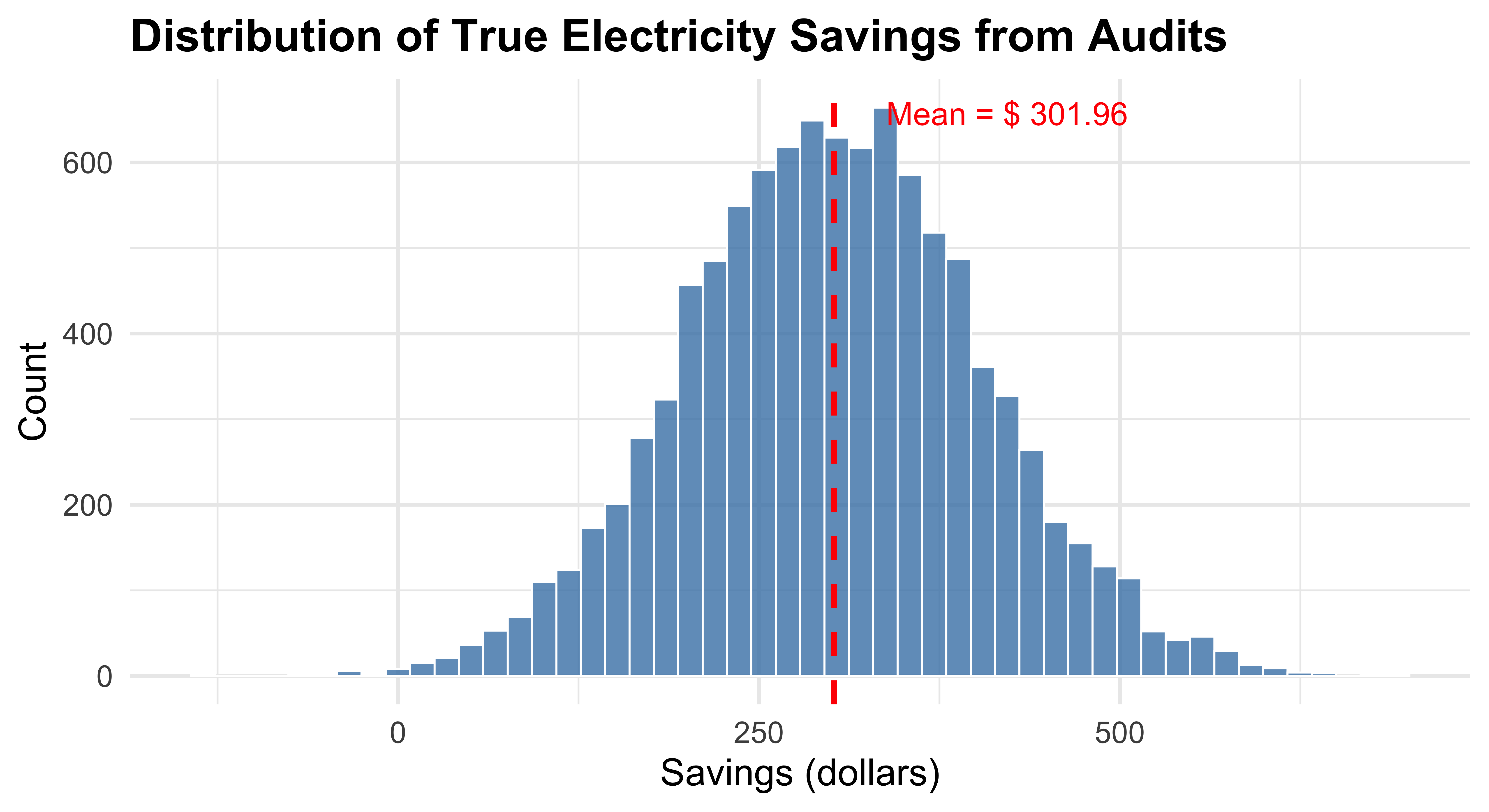
Average savings across all households if audited: $301.96

This is the true population average treatment effect.

Distribution of Savings

Treatment effects are heterogeneous: some households save a lot, some very little.

Question 2: Voluntary Opt-in

Who Chooses Audits?

Setup (same model as “Who selects into audits?” in lecture):

  • Audits cost $250
  • Households have hassle costs (time, effort)
  • Households form expectations about savings

Decision Rule: Get an audit (\(A_i = 1\)) if: \[\text{Expected Savings} > \$250 + \text{Hassle Cost}\]

Calculate: Net savings = \((\text{ey}_{10} - \text{ey}_{11}) - \text{hassle} - 250\)

Opt-in Analysis

Show code
# Calculate expected savings and net savings
audit_data <- audit_data %>%
  mutate(
    exp_savings = ey10 - ey11,
    net_savings = exp_savings - hassle - 250,
    D_optin = if_else(net_savings > 0, 1, 0)
  )

# Count opt-ins
optin_count <- sum(audit_data$D_optin)

# Average treatment effect by group
ate_by_group <- audit_data %>%
  group_by(D_optin) %>%
  summarise(
    n = n(),
    avg_savings = mean(savings),
    avg_exp_savings = mean(exp_savings),
    avg_net_savings = mean(net_savings),
    .groups = "drop"
  )

ATT <- ate_by_group$avg_savings[ate_by_group$D_optin == 1]
Treatment Effects by Opt-in Status
Group N Avg Savings Avg Expected Savings Avg Net Savings
Don't opt-in 6488 254.56 233.61 -120.35
Opt-in 3512 389.53 429.77 87.58

Key Insight: Selection

Selection into Treatment

  • 3512 households opt in voluntarily
  • Opt-in group has higher average savings ($389.53)
  • Non-opt-in group has lower average savings ($254.56)

Why? People who benefit more are more likely to opt in!

The average savings for the opt-in group is the average treatment effect on the treated (ATT).

Question 3: Naive Comparison

Naive Comparison

The tempting approach: Compare people who got audits to those who didn’t

Show code
# Create observed outcome variable
audit_data <- audit_data %>%
  mutate(y1obs = if_else(D_optin == 1, y11, y10))

# Calculate means by group
cross_section <- audit_data %>%
  group_by(D_optin) %>%
  summarise(
    mean_y10 = mean(y10),
    mean_y11 = mean(y11),
    mean_y1obs = mean(y1obs),
    .groups = "drop"
  )

# Naive estimate: non-audited minus audited spending
est_xsection <- cross_section$mean_y1obs[1] - cross_section$mean_y1obs[2]
Mean Outcomes by Opt-in Status
Group Mean Y10 Mean Y11 Mean Observed Y
Don't opt-in 1979 1724 1979
Opt-in 2034 1645 1645

Naive difference: $334 vs. True ATE: $302 vs. True ATT: $390

Decomposing the Naive Comparison

In savings terms: naive comparison = ATT − selection bias.

\[ \begin{aligned} \underbrace{E[Y_{i0}\mid A_i=0] - E[Y_{i1}\mid A_i=1]}_{\text{naive}} &= \underbrace{E[Y_{i0} - Y_{i1}\mid A_i=1]}_{\text{ATT}} \\ &\quad - \underbrace{\left(E[Y_{i0}\mid A_i=1] - E[Y_{i0}\mid A_i=0]\right)}_{\text{selection bias}} \end{aligned} \]

Our special data reveal every piece

  • ATT: $390
  • Selection bias: $2034 (opt-ins) − $1979 (others) = $55
  • Naive: $390 − $55 = $334

Opt-ins use more energy without audits, biasing naive savings downward.

Can we just run a regression?

With a single audit dummy, OLS gives the same biased answer:

\[Y_i^{\text{obs}} = \alpha + \beta A_i + \varepsilon_i\]

Here \(A_i = 1\) if household \(i\) opts in (D_optin).

OLS: observed spending on opt-in dummy
term estimate std.error statistic p.value
(Intercept) 1979.0 2.1 935.6 0
D_optin -334.3 3.6 -93.7 0
  • Coefficient on D_optin = −(naive difference)
  • \(A_i\) is correlated with the error term: omitted variable bias
  • Controls still miss unobserved expectations and hassle costs

Question 4: Randomized Experiment

The Gold Standard: RCT

Setup:

  • Randomly select 1,000 households
  • Force them to have audits (treatment group)
  • Remaining 9,000 households = control group
  • Compare outcomes

Key: Randomization makes the selection bias term zero (in expectation)

RCT Implementation

Show code
# Randomize treatment assignment
audit_data <- audit_data %>%
  mutate(irand = runif(n())) %>%
  arrange(irand) %>%
  mutate(D_treat = if_else(row_number() <= 1000, 1, 0))

# Calculate means for treatment and control
rct_means <- audit_data %>%
  group_by(D_treat) %>%
  summarise(
    mean_y10 = mean(y10),
    mean_y11 = mean(y11),
    .groups = "drop"
  )

# Estimate from experiment: control Y0 minus treated Y1
est_experiment <- rct_means$mean_y10[1] - rct_means$mean_y11[2]

RCT Results

RCT: Mean Outcomes by Treatment Status
Group Mean Y10 Mean Y11
Control (no audit) 1998 1696
Treatment (forced audit) 2003 1699

Result

  • RCT estimate: $299
  • True ATE: $302

Very close! Small difference due to sampling variation.

Mean Y10: Both groups would spend about the same without an audit: no selection bias.

Question 5: Free Audits (No Mandate)

Realistic Policy: Encouragement, Not Mandates

Problem: Can’t actually force people to get audits!

New Setup:

  • Same 1,000 randomly selected households get free audits
  • Other 9,000 can still pay $250 for audits
  • Households choose whether to accept

Key Change: Randomize the offer (\(Z_i\)), not the audit itself (\(A_i\)). This is the random encouragement design from lecture.

Who Takes Up Free Audits?

Show code
# Calculate net savings with RCT (free audits for treatment group)
audit_data <- audit_data %>%
  mutate(
    net_savings_rct = if_else(D_treat == 1,
                              net_savings + 250,  # No cost for treatment
                              net_savings),       # Still costs $250 for control
    D_optin_rct = if_else(net_savings_rct > 0, 1, 0)
  )

# New opt-ins
new_optins <- sum(audit_data$D_optin_rct == 1 & audit_data$D_optin == 0)
total_optin_rct <- sum(audit_data$D_optin_rct)

Takeup

  • Original opt-ins (at $250): 3512
  • Opt-ins with free audits for the treatment group: 4112
  • Screened in by free audit: 600 households

The free offer increases participation by 17%!

Question 6: Intent-to-Treat

Intent-to-Treat (ITT)

Definition: Compare outcomes based on random assignment (\(Z_i\)), not actual behavior (\(A_i\))

  • Treatment group = offered free audit
  • Control group = not offered free audit

Why? Preserves randomization even with imperfect compliance

Show code
# Create observed outcome under RCT
audit_data <- audit_data %>%
  mutate(y1obs_rct = if_else(D_optin_rct == 1, y11, y10))

# Calculate ITT
itt_means <- audit_data %>%
  group_by(D_treat) %>%
  summarise(mean_y1obs_rct = mean(y1obs_rct), .groups = "drop")

# ITT estimate
est_itt <- itt_means$mean_y1obs_rct[1] - itt_means$mean_y1obs_rct[2]

ITT Results

Intent-to-Treat: Mean Outcomes
Group Mean Electricity Spending
Not offered 1861
Offered free audit 1704

Much Smaller Effect!

  • ITT estimate: $157
  • True ATE: $302

Many households in both groups get audits. The offer changes behavior only for some.

Question 7: Local Average Treatment Effect

Defining Compliers

Three types of households (as in lecture):

  1. Always takers: Would get an audit even at $250
  2. Compliers: Only get an audit when it’s free
  3. Never takers: Don’t get an audit even when free

Key insight: The encouragement only changes behavior of compliers!

Identifying Compliers

Show code
# Identify compliers
audit_data <- audit_data %>%
  mutate(compliers = if_else(D_optin_rct == 1 & D_optin == 0, 1, 0))

# Compliance rates by treatment group
compliance_table <- audit_data %>%
  group_by(D_treat) %>%
  summarise(
    n = n(),
    pct_optin_rct = mean(D_optin_rct) * 100,
    pct_optin_original = mean(D_optin) * 100,
    pct_compliers = mean(compliers) * 100,
    .groups = "drop"
  )

# Complier share and LATE
comply_share <- mean(audit_data$compliers[audit_data$D_treat == 1])
est_late <- mean(audit_data$savings[audit_data$compliers == 1])
never_share <- mean(audit_data$D_optin_rct[audit_data$D_treat == 1] == 0)
always_share <- mean(audit_data$D_optin[audit_data$D_treat == 1])

Compliance Rates

Compliance Rates by Treatment Assignment
Group N % Opt-in (RCT) % Opt-in (at $250) % Compliers
Control 9000 35.0 35.0 0
Treatment 1000 95.8 35.8 60

Key Numbers

Shares of the treatment group:

  • Always takers: 35.8% · Compliers: 60% · Never takers: 4.2%
  • LATE (savings for compliers): $268
  • Compare to ATE: $302

Why is LATE < ATE?

Compliers (free audit only):

  • Lower expected savings
  • Higher hassle costs
  • On the margin

Average savings: $268

Always takers (pay $250):

  • Higher expected savings
  • Lower hassle costs
  • Inframarginal

Average savings: $390

Households with highest benefits adopt first!

Question 8: The ITT-LATE Connection

The Formula

Relationship (from lecture): \[\text{ITT} = \text{Share of compliers} \times \text{LATE}\]

Intuition:

  • Always takers get audits in both groups, never takers in neither: they cancel out
  • Only compliers are treated differently across the two groups
  • So the ITT is the compliers’ savings, diluted by everyone else

Verification

Show code
# Check ITT = compliance_rate * LATE
predicted_itt <- comply_share * est_late

The Math Checks Out (up to sampling variation)

  • Share of compliers: 0.6
  • LATE: $267.66
  • Predicted ITT: 0.6 × $267.66 = $160.59
  • Actual ITT: $156.79

Not exact: the always takers in the control group are a different random sample than those in the treatment group.

What can an econometrician estimatate?

We used unobserved hassle costs and expectations to identify compliers. A regulator can observe:

  • Average spending in each randomized group → ITT
  • Audit rates in each randomized group → share of compliers

\[\text{LATE} = \frac{E[Y|Z_i=1]-E[Y|Z_i=0]}{Pr(A_i=1|Z_i=1)-Pr(A_i=1|Z_i=0)}\]

  • Audit rate: 95.8% (offered) − 35% (not offered) = 60.8%
  • Observable LATE: $157 / 0.608 = $258
  • True complier savings: $268; the gap is sampling variation

Question 9: Policy Implications

Which Estimate Should We Use?

ATE ($302):

Use if you can:

  • Mandate participation
  • Achieve universal coverage
  • Don’t care about costs

Problem: Infeasible and ignores heterogeneity

LATE ($268):

Use for:

  • Voluntary programs
  • Subsidies/incentives
  • Marginal participants

Advantage: Estimates effect on those you’ll actually influence

Key Policy Insights

Main Takeaways

  1. Heterogeneous treatment effects: Benefits vary across households

  2. Selection matters: Those who benefit most adopt first

  3. Declining returns: Each additional adopter has lower savings

  4. Cost-benefit analysis: Optimal policy stops before 100% adoption

  5. Target the margin: Focus on compliers, not always takers

Summary

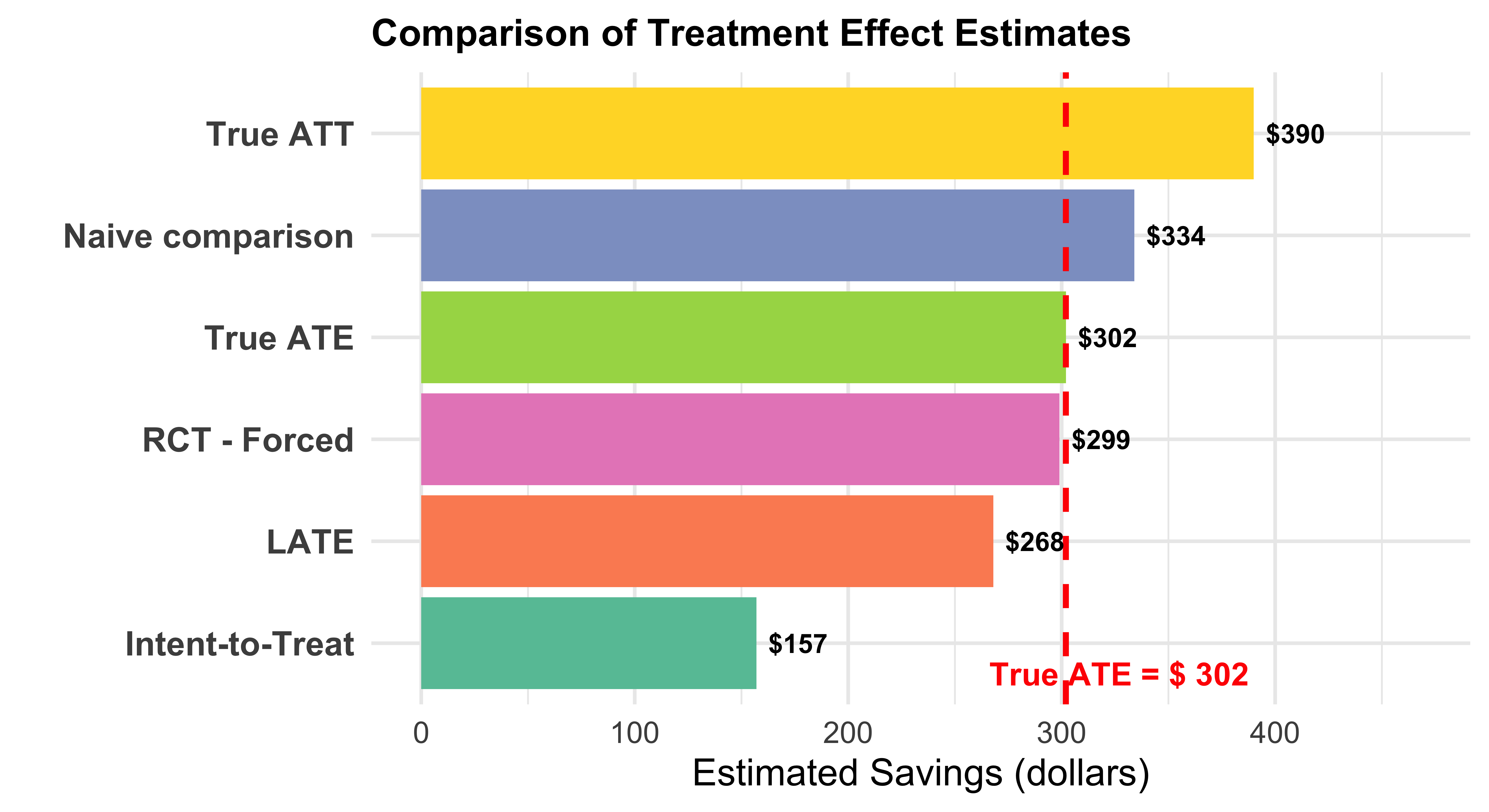
Comparison of All Estimates

Summary of Treatment Effect Estimates
Method Question Estimate Notes
True ATE 1 302 Everyone
True ATT 2 390 Voluntary adopters
Naive comparison 3 334 Selection bias
RCT - Forced 4 299 None (forced)
Intent-to-Treat 6 157 Diluted by always/never takers
LATE 7 268 Compliers only

Visual Comparison

Lessons for Policy Evaluation

  1. Naive comparisons mix the causal effect with selection bias

  2. Randomization eliminates selection bias (when compliance is perfect)

  3. ITT preserves randomization with imperfect compliance

  4. LATE identifies effect on marginal participants, and can be recovered as ITT / share of compliers

  5. Choose estimand based on policy: What question are you trying to answer?

Final Thoughts

The Big Picture

Energy efficiency programs face fundamental challenges:

  • Private information: Households know their benefits best
  • Selection on gains: Highest-benefit households adopt first
  • Diminishing returns: Wider participation lowers average benefits
  • Optimal policy ≠ universal adoption

Good policy evaluation requires understanding who is affected by your intervention!

Up Next: A Real Encouragement Experiment

Fowlie, Greenstone & Wolfram: The Weatherization Assistance Program in Michigan

  • Randomly encouraged 25% of eligible households to weatherize
  • Weatherization was free, yet take-up was only 6% (encouraged) vs. 1% (control)
  • Same tools as this homework: ITT, compliers, LATE

Questions?

Appendix

Distribution of Hassle Costs

Hassle costs (\(\xi\)) capture the time and effort of undergoing an audit.