Introduction
Agenda
-
Introductions
- Basics of environmental economics theory
- for more see Baumol \& Oates
- Overview of some key questions and the frontier of research
- Emphasis on IO, see Kellogg \& Reguant
- Goal is to get you thinking about the research frontier
Environmental Economics Theory
Environmental economics is essentially the study of externalities
An externality is something that enters into the utility (or production) function of one agent but is chosen by another agent.
Classic example is something that enters directly:
- a neighbor’s loud music
Externalities can also enter indirectly/ alter consumption sets
- right now PM from wildfires is keeping some people indoors
However an important distinction is made between those cases and situations where the actions by one agent affect another’s utility through prices (a pecuniary externality)
- for example if demand for short term rentals on AirBnB drives up rents and makes housing less affordable for some residents
Another classic example is the case of mutually beneficial production externalities
Meade (1952) considered the case of a beekeeper and nearby orchard.
- Bees pollinate the orchard, and the orchard nourishes the bees, shifting the production possibilities of both businesses outward
A formal model of production externalities
Setup
-
two individuals $i \in (1,2)$ receive utility from private goods $x$ and $z$ and disutility from emissions $E$
- $x$ is a dirty good produced using labor $l$ and emissions
- $x = f(l_x,E)$, with $df(E)/dE>0$
- clean good $z$ produced only using labor: $g(l_z)$
- labor in economy constrained by time endowment $l$
[familiar FOCs below]
Find Pareto optimal allocation by maximizing $U_1$, holding $U_2$ at some reference level
Efficiency in consumption
Marginal rate of substitution equal for both individuals
\[\frac{\partial U_1()/\partial x_1}{\partial U_1()/\partial z_1} = \frac{\lambda_x}{\lambda_z} = \frac{\partial U_2()/\partial x_2}{\partial U_2()/\partial z_2}\]Marginal product of labor equal to the shadow value on labor constraint in both markets
\[\lambda_x \frac{\partial f()}{\partial l_x} = \lambda_l = \lambda_z \frac{\partial g()}{\partial l_z}\]Exchange efficiency sets slope of production possibility curve equal to slope of each individual’s indifference curve
\[\frac{\partial U_i()/\partial x_i}{\partial U_i()/\partial z_i} = \frac{\lambda_x}{\lambda_z} = \frac{\partial g()/\partial l_z}{\partial f()/\partial l_x}\]Now look at the optimality condition for emissions
Reducing $E$ increase utility for both people directly, but decreases their utility indirectly by reducing $x$ consumed.
- Net effect depends on preferences.
Taking the FOC wrt $E$, and rearranging yields
\[- \left[ \frac{\partial U_1()/\partial E}{\partial U_1()/\partial x_1} + \frac{\partial U_2()/\partial E}{\partial U_2()/\partial x_2} \right] = \frac{\partial f()}{\partial E}\]Optimal $E$ equates the sum of each individuals marginal willingness to tradeoff $E$ for $x$ with the physical reduction in $x$ production induced by changing $E$
- Here $E$ is not just an externality but also a public good
We can then compare this Pareto outcome to the competitive market
- Define prices $p_z$ and $p_z$, wage $w$, and income $y_i$
- Firms and individuals act as price takers
Individuals max \(Max_{x_i,z_i} \hspace{5pt} U_i(x_i,z_i,E) + \lambda_i[y_i - p_x x_i - p_z z_i]\)
Firms producing $x$ and $z$ max \(Max_{l_x,E} \hspace{5pt} p_x f(l_x,E) - w l_x\)
\[Max_{l_z} \hspace{5pt} p_z g(l_z) - wl_z\]While the efficiency in labor use and exchange conditions are met, the emission allocation is no longer efficient
\[p_x \frac{\partial f()}{\partial l_x } = w\] \[p_x \frac{\partial f()}{\partial E } = 0\]Firms face zero marginal cost of $E$ and use too much of it.
Pigou (1920) noted that optimality could be restored with a tax
Pareto: \(- \left[ \frac{\partial U_1()/\partial E}{\partial U_1()/\partial x_1} + \frac{\partial U_2()/\partial E}{\partial U_2()/\partial x_2} \right] = \frac{\partial f()}{\partial E}\) Consider tax $\tau$, so \(\pi = p_x f(l_x,E) - w l_x - \tau E\)
Pigouvian tax: \(\tau = -p_x \bigg[ \frac{\partial U_1()/\partial E}{\partial U_1()/\partial x_1} + \frac{\partial U_2()/\partial E}{\partial U_2()/\partial x_2} \bigg]\)
Coase (1960) challenged whether this was actually necessary
Example:
- Baker and a doctor share a wall.
- The baker installs a machine which causes vibrations, impairing the doctor’s ability to operate.
Pigou:
Efficiency restored by taxing baker at dentists marginal harm from vibrations.
Coase’s challenge
-
Unclear who’s imposing the externality on who
-
Efficient outcome could also be achieved by if dentist offers payment up to his marginal harm for baker to quit using the machine.
- challenge to “polluter pays”
Colloquial conclusion:
- Doesn’t matter who has the property rights, as long as their well defined, efficient outcome will obtain
Coase Theorem requires three assumptions
- Well defined property rights
- No transaction costs
- No income / endowment effects
These conditions (mainly 2) rarely satisfied in the real world
- starting point for theory of the firm (Williamson)
More recently, Myerson-Satterthwaite theorem casts further doubt on viability of property rights alone to efficiently adjudicate externalities
- No good way for two parties to trade a good when they each have secret valuations
Other policy options
Most environmental regulations are not Pigouvian taxes, but “command and control”.
- Government sets emission limits or rates by facility.
- How does this compare to Pigouvian solution?
A simpler model
Household utility: $U_i(y_i,E)= y_i - D_i(E)$
Summing over $i$ yields the damage function: $D(E)=\sum_i D_i(E)$
Firms can abatement emissions at cost $C_j(e_j)$
- these include full opportunity costs (not just direct costs)
- $C_j(\hat{e_j}) = 0$ at unregulated level.
Social net benefits of pollution = $\sum_j C_j(e_j) - D(E)$
Efficient allocation equates marginal damages with marginal abatement costs at all firms
\[C'_j(e_j) = D'(E) \hspace{15pt} \forall j=1,..J\]Therefore, the marginal cost of each polluter are also equal
\[C'_j(e_j) = C'_k(e_k) \hspace{15pt} \forall j,k\]This is a necessary and sufficient condition for cost-minimization of any policy (such policies are “cost effective”)
Pigovian taxes achieve this by construction: \(C'_j(e_j) = \tau \hspace{15pt} \forall j=1,..J\)
Regulation unlikely to be cost effective in practice
-
If regulator knows all the $C_j$’s, could chose $e_j$ appropriately
-
In practice, such regulations never firm specific
- Cost effectiveness only achieved if all polluters are identical
More importantly, regulator doesn’t actually know $C$
- tax cost effective by construction
- but command and control requires full information
Another option: Cap-and-trade
- Regulator issues a fixed amount of emission permits $\bar Q$
- Assume these are auctioned off, with clearing price $\rho$
Firm’s minimize total compliance costs:
\(TC_j(e_j) = C_j(e_j) - \rho e_j\) \(s.t. \sum_j e_j \leq \bar{Q}\)
Assuming firms are price takers,
\[C'_j(e_j) = \rho \hspace{15pt} \forall j=1,..J\]Prices vs Quantities
In static world of full information (ie known MC and MD), taxes and allowances are equivalent
- Note: If permits aren’t auctioned, Coase independence assumptions apply.
Weitzman (1974) considered efficiency when there is uncertainty about the damage or cost functions.
- Assume planner must set policy based on expected MB and MC, and then true functions materialize
Prices vs Quantities: Steep MC
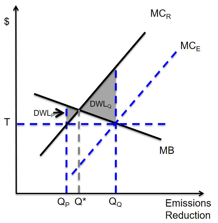
Prices vs Quantities: Steep MB
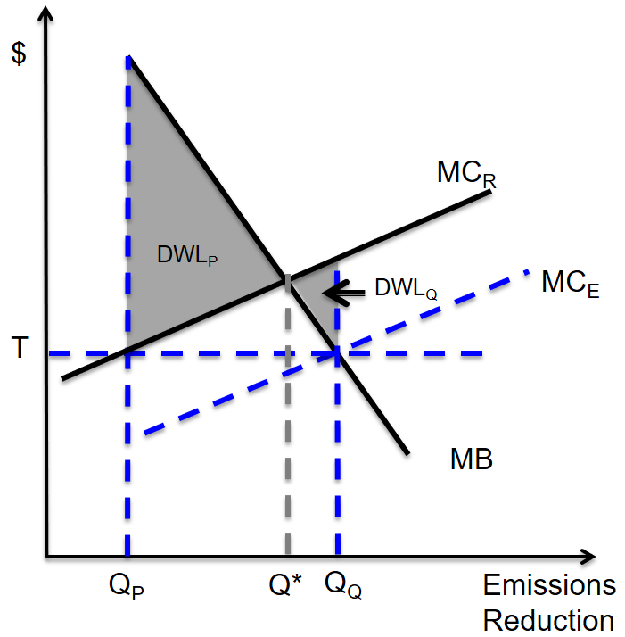
Summary of results: the Weitzman Rule
- If costs are uncertain and slope of MB > MC, use quantity instrument
- If costs are uncertain and slope of MB < MC, use price instrument
Intuition: Gradient tells you how bad it is to be wrong in each direction.
- Surprising result: If only MB are uncertain, instruments are equivalent (equally bad)
Intuition: pollution chosen by firms setting $MC = \tau$ or $\rho$. If costs don’t change, resulting marginal prices don’t change, and expected $E$ obtained.
Stavins 1996 considers correlated uncertainty.
Seems likely that uncertainty in MB and MC are positively correlated.
If that’s the case, quantity instrument becomes more appealing (can see this visually)
Roberts and Spence (1976) show a hybrid instrument can outperform either
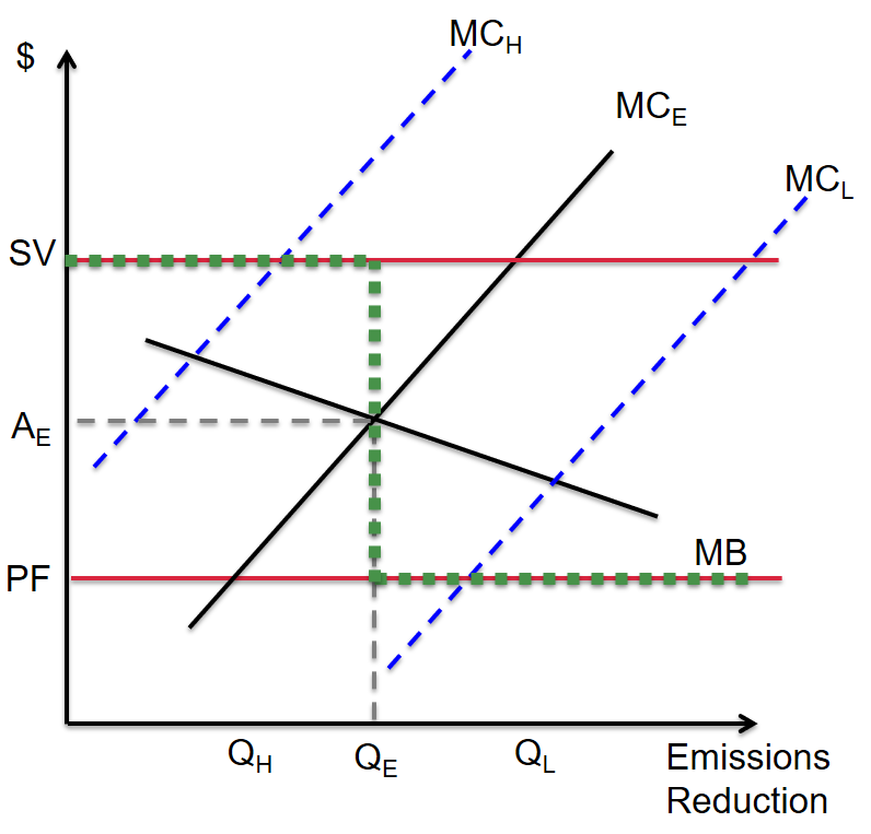
Most recent cap-and-trade policies have included a price bounds
- Politically ceiling helpful assuaging business community fears
- Floor also increasingly important for environmental stakeholders
What is the active research in this area?
-
Some work on details of cap and trade, particularly over long run
- Lots of work over past decade tests core predictions:
- Are outcomes independent of allocation?
- Is C&T cost-effective?
- But more interesting is how these theoretically first-best policies compare to what’s done in practice.
- Many policies contain elements that are not well motivated (economically)
- Carve outs; Grandfathering;
- What the costs of these?
-
Particularly important is overlapping policy instruments:
- MA participates in a regional Co2 cap-and-trade program AND mandates a minimum level of renewable energy.
-
We’ll also spend time looking at common alternative policies:
- Behavioral interventions (nudges)
- Subsidies
Probably the largest area of research involves estimating costs and benefits
-
If policy maker wanted to set the optimal tax, what should it be?
- Bulk of these papers estimate health (or related) impacts
- mortality and morbidity
-
Then use benefit transfer to convert to $
- More recently people have linked to intermediate outcomes of obvious policy interest
- test scores (Goodman et al 2018)
- worker productivity (Zivin & Neidel 2011)
Where possible economists still prefer to use revealed preference methods
As opposed to benefit transfer to assign value.
We’ll spend a week on the workhorse model in this area: hedonic property valuation.
- Great example of reduced form vs structural approach to EE
- Interesting overlap with behavioral
This course will largely focus on firm side of EE
- polluting markets often characterized by imperfect competition
- multiple market failures –> actual DWL unclear
- market power complicates firm response to simple models presented above
- dynamics
- innovation
- behavioral!
IO tools well suited to recover preferences and run counterfactuals
What does the frontier of this literature look like?
[hopefully your term paper, eventually]
- Test a theory
- tough to find low hanging fruit
- i.e. independence of allocation
- Measure costs and benefits
- identification
- SUTVA / spillovers
- something we don’t know about (like fine PM)
- some important extension: long vs short run; avoidance - adaptation; behavioral
- climate change per se important (but crowded)
- identification
- Evaluate a policy
- not enough unless you tie to theory/ some broader question
- compare second (third..) best to ideal policy
- “dumb” policies often provide nice experiments to test other hypotheses
- Environmental settings are good for learning about economics more broadly
- Hunt’s papers
- Energy markets have nice properties (undifferentiated, clear mechanisms, good data, lots of policy )