Lecture draws on:
Allcott and Greenstone (JEP 2012)
Allcott (Annual Review 2014)
Gerarden, Newell and Stavins (JEL 2018)
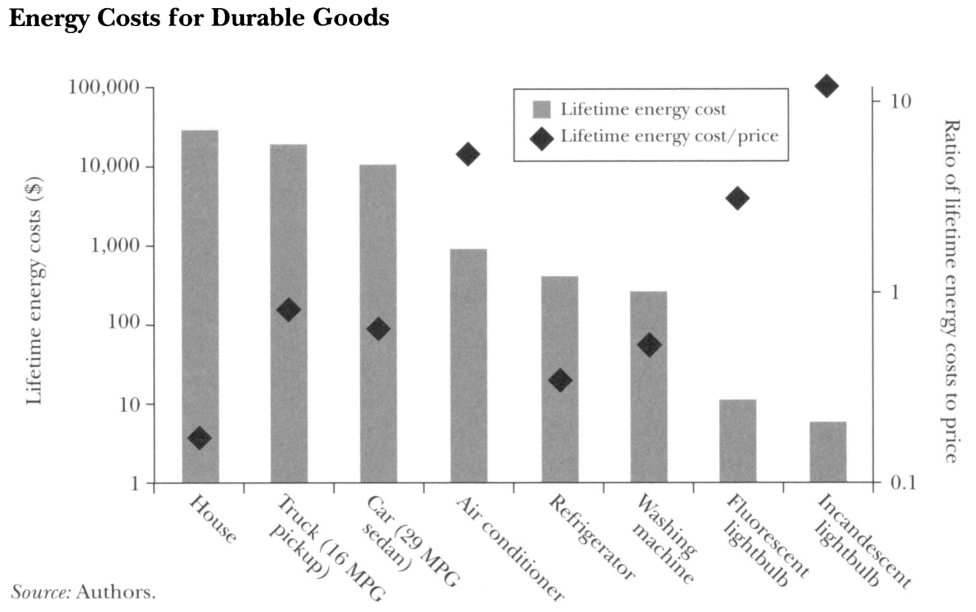
Long standing assertion that energy efficient capital suboptimally deployed
Over time interest has centered on apparent "win-win" from environmental perspective
- Energy consumption associated with many externalities
-
agency issues
-
resale issues
-
engineering models wrong
[from Allcott (2014)]
Consumers have indirect utility
$$u_{j} = \eta (y - p_j - \gamma g_j) + \nu_j$$
- $p_j$ is upfront cost
- $\nu_j$ is the usage utility
- $g_j$ is the lifetime energy cost
Assuming $g$ is calculated and discounted appropriately, a natural test is to estimate $\gamma$ and test if its equal to 1.
$$g_{j} = \sum\limits_{t=0}^{T} \delta^t m(r_j,e_t)r_j e_t$$
- $m$ is utilization
- $r_j$ is energy requirement for capital $j$
- $e$ is the energy price
Note
- $\delta, m, T, e$ could all have $i$ subscripts
- if $m$ is endogenous, can lead to a "rebound effect"
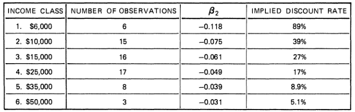
Hausman (1979) estimates a discrete choice model for AC's
$$u_{ij} = \eta (y_i - p_j - \delta_i \bar m_i r_j e_t) + \alpha X_j + \epsilon_{ij}$$
- Has a small survey of households with submetered ACs
- In the cross section, concern that $E[r_j \epsilon_j] \ne 0$
However, $g_{ij}$ varies for many other reasons within product
- energy prices vary
- lifetime varies at time of sale
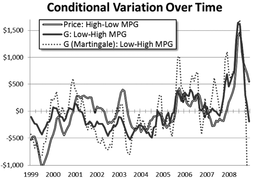
- Sallee et al. look at mileage
Allcott and Wozny
ReStat (2014)
- What's the research question?
- What's the empirical strategy?
- What data do they have?
$$p_{j} + \sum\limits_{t=0}^{T} \delta^t m(r_j,e_t)r_j e_t$$
- used car auction vehicle prices from Manhiem
- what are the assumptions using this?
- assumed real discount rate of 6%
- vehicle loan rate 6.9%
- S&P avg return 5.9%
- (exogenous) VMT ($m$) and $T$ from NHTSA
- fuel economy from EPA
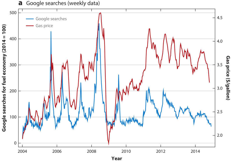
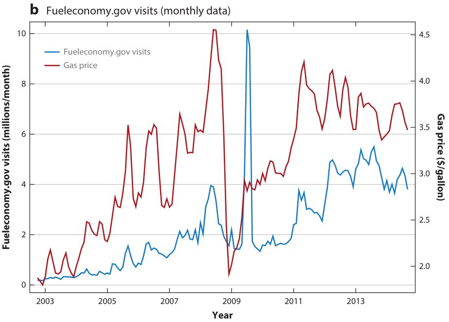
- national avg gasoline prices / oil futures
Typical logit share identity (Berry, 1994):
$$\ln s_{jat} - \ln s_{ot} = -\eta (p_{jat} - \gamma g_{jat}) + \psi_{ja} + \tilde \xi_{jat}$$
AW actually estimate:
$$p_{jat} = - \gamma g_{jat} + \tau_t + \psi_{ja} + \epsilon_{jat}$$
Why do they do this?
Berry equation rearranged is
$$p_{jat} = - \gamma g_{jat} - \frac{1}{\eta}(\ln s_{jat} - \ln s_{ot} ) + \psi_{ja} + \tilde \xi_{jat}$$
- The don't have shares.
- Absorb $s_{ot}$ with time FEs.
- Put product FEs in $\psi_{ja}$
- $\xi$ and the remaining share difference in the $\epsilon$
$$p_{jat} = - \gamma g_{jat} + \tau_t + \psi_{ja} + \epsilon_{jat}$$
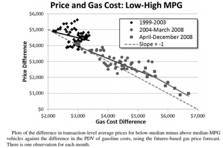
- So this tests it tests whether relative vehicle prices move one-for-one with changes in the relative gasoline costs.
- Coeff of interest $\gamma$ recovered with OLS.
Jerry Hausman's (2001) "iron law of econometrics": due to measurement error, the magnitude of a parameter estimate is usually smaller in absolute value than expected
What is the null hypothesis that AW want to test?
$$p_{jat} = - \gamma g_{jat} + \tau_t + \psi_{ja} + \epsilon_{jat}$$
-
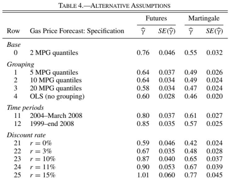
tradeoff implies discount rate of about 15%
- for new cars, close to 1
- old cars, very low
-
results sensitive to how G is constructed
-
are people making mistakes?
-
what questions does this leave open?
-
Many studies similar to AW
-
Although panel data helps, interpretation still requires econometrician to construct $g$
-
If hypothesis is that $\gamma < 1$ due to inattention, imperfect information or bounded rationality, an alternative is to experimentally vary exactly those margins
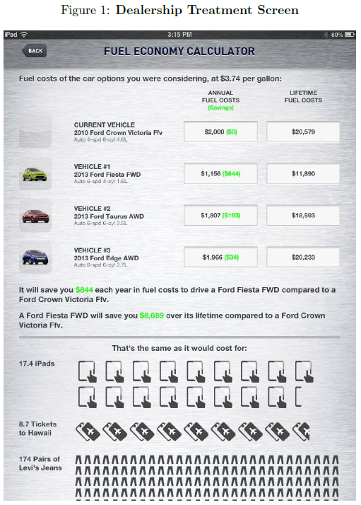
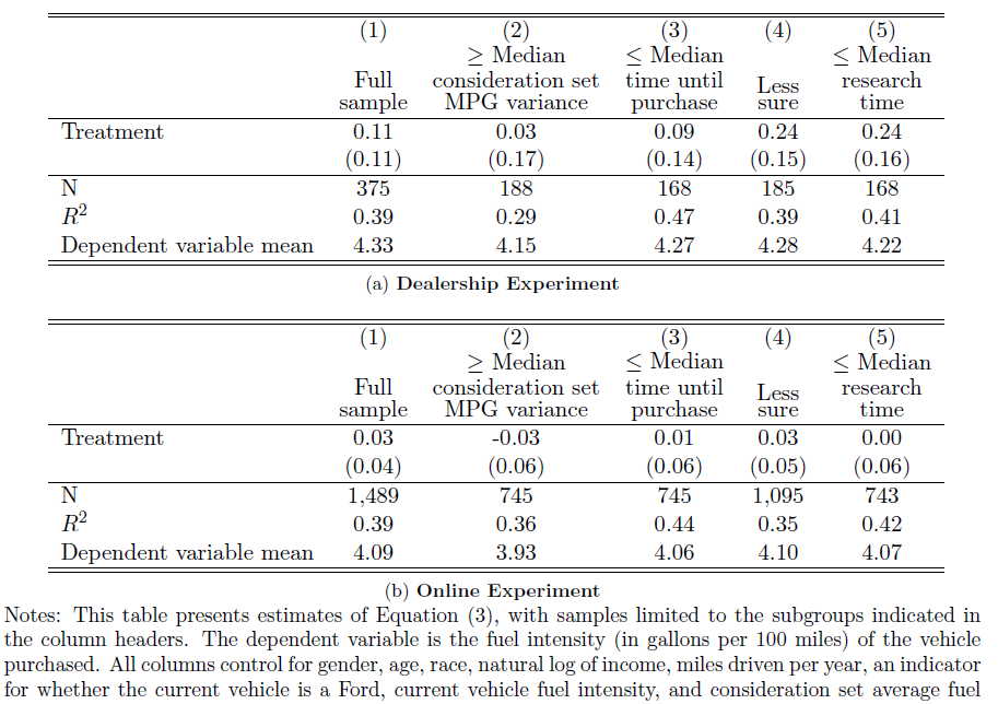
Experiment #1:
- Hang out at car dealers and intercept potential buyers
- Randomly explain fuel economy savings to some
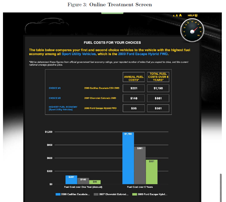
Experiment #2:
- Conduct and online survey of people how say they are in the market for a new car
- In addition to following up on what people actually bought, AK elicit WTP for fuel economy.
-
assertion that consumers making large mistakes on average appears incorrect
-
once you account for product unobservables and use exogenous fuel cost variation, tradeoffs seem close to rational
-
experimental studies directly educating or directing consumer attention to energy costs have found very small impacts
-
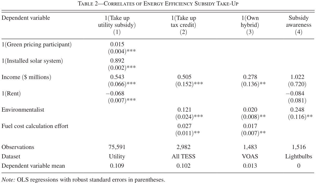
Heterogeneity in both values and bias
- policy implications
- targeting
-
What role do firms play here?
- Are they offering the "right" set of products?
-
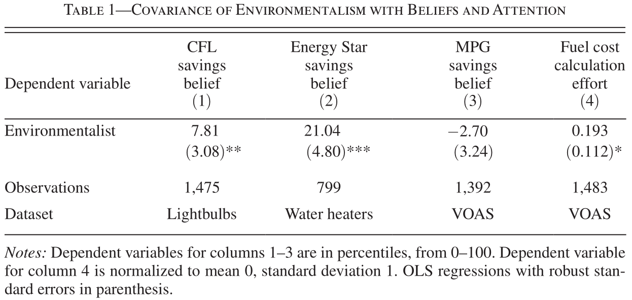
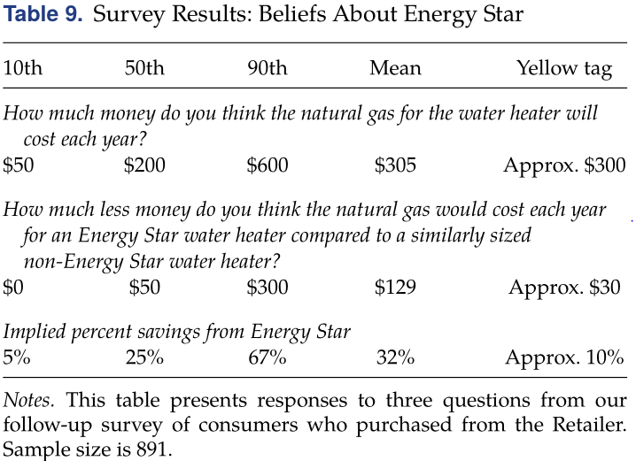
How do consumer's form beliefs?
- we know the true calculation is hard
-
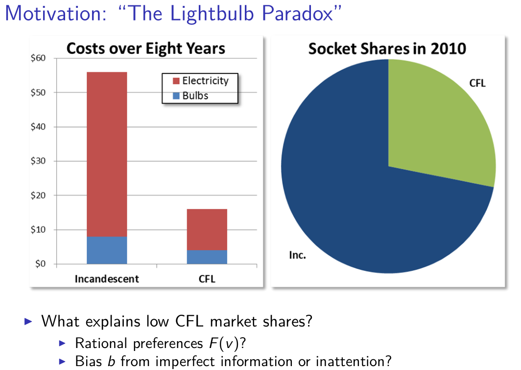
develop a theoretical framework in presence of heterogenous bias and tastes
-
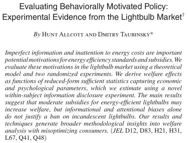
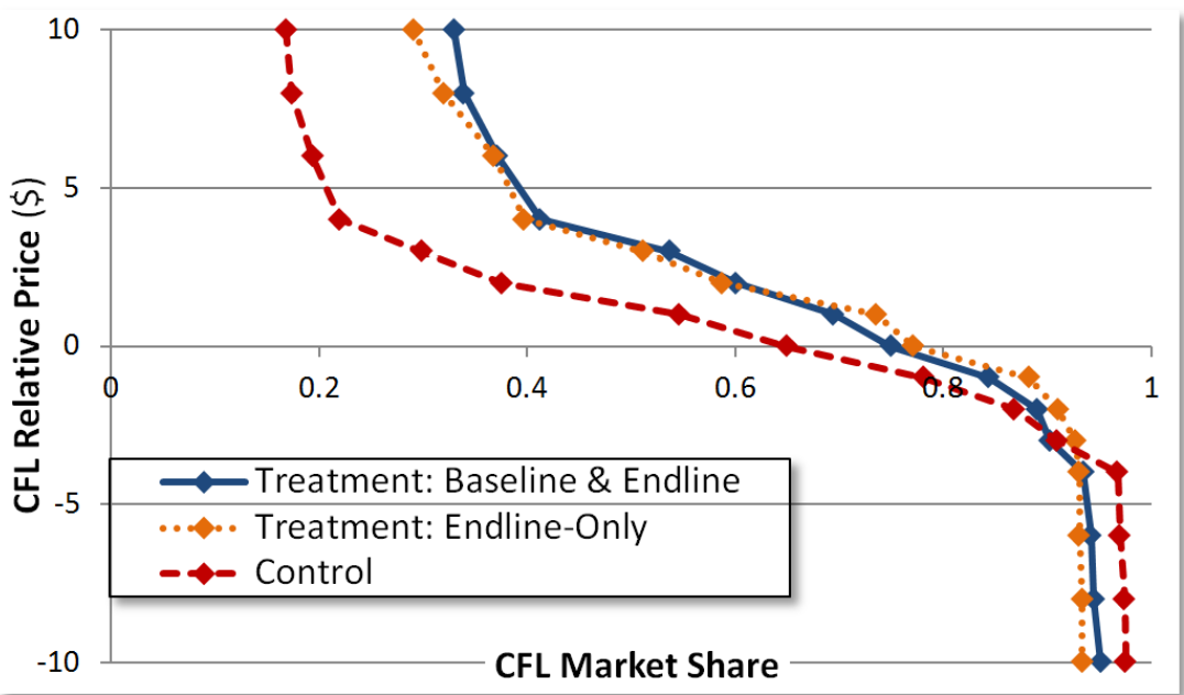
implement two experiments informing consumers about CFLs
-
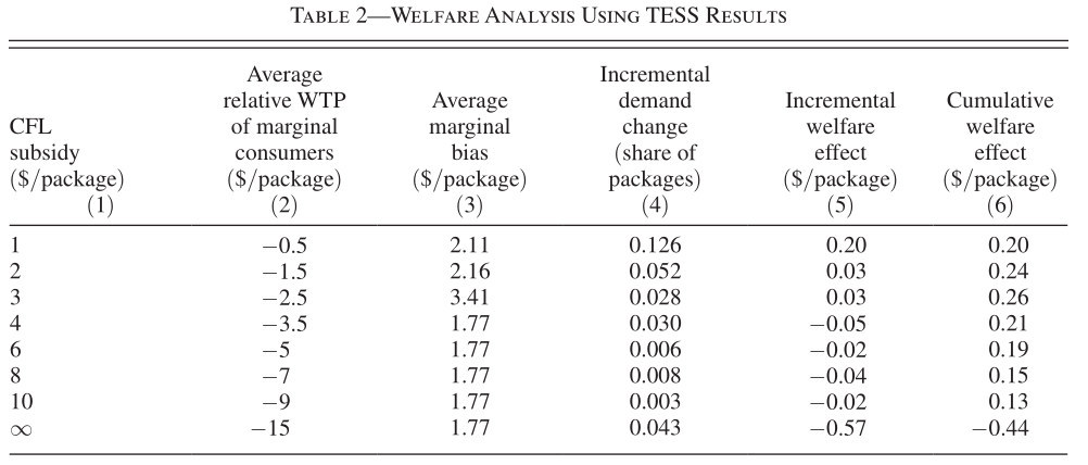
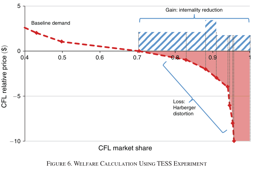
evaluate welfare effects:
- optimal subsidy
- [ban on incandescents]
Pigou (1920):
$$\tau = D'(e)$$
If damages are heterogenous, first best achieved with polluter specific tax
$$\tau_i = D_i'(e_i)$$
Diamond (BJE 1973): If damages are heterogeneous, but you can only set one tax rate, it should be equal to the average damages at the margin when the tax is implemented.
$$\tau_h = E_i[ D'_i(e_i(\tau_h))]$$
Setup
-
unit demand: $j \in {E,I}$
-
utility: $u_j = v_j + z - P_j$
- where $z$ is the consumer's budget
-
choose $E$ if $v - b > p$
- $v = v_E - v_I$
- $b$ is bias
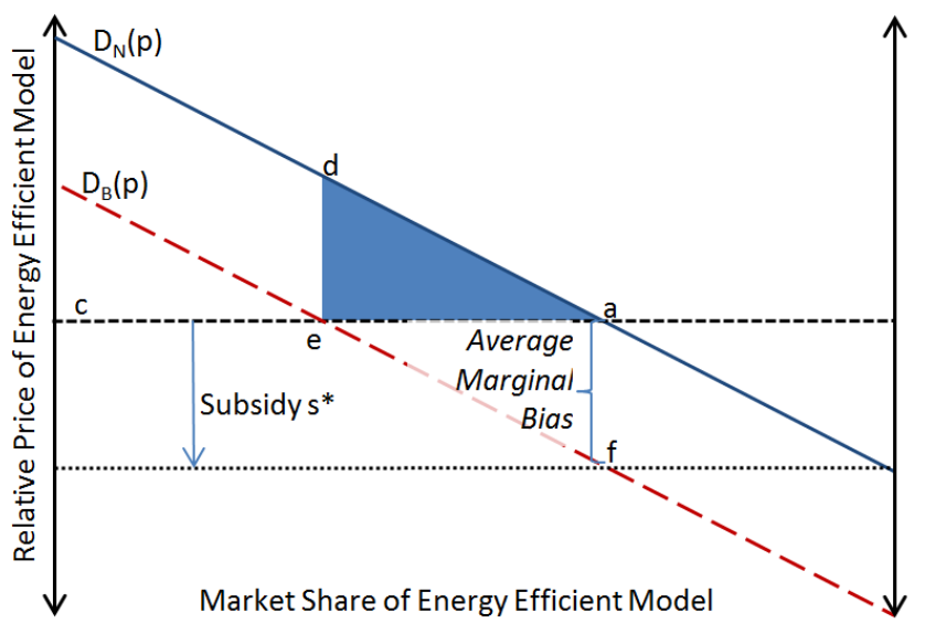
Demand with and without bias
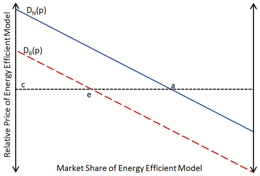
$$W(s) = Z(s) + v_I - p_I + \int_{v-b \ge p}(v - p) dF dG$$
- perfect competition: $p = c - s$
Proposition 1:
$$W'(s) = (s - B(p)) D'_B(p)$$
where $B = E(b|v - b = p)$ is the average marginal bias -- ie the average bias for consumers on the margin the (subsidized) price
Optimal subsidy:
$$s^* = B(c - s^*)$$
Need not be constant
- Average marginal bias $\ne$ average bias
How can we estimate the average marginal bias?
Option 1:
- use within consumer variation in informedness
Option 2:
- estimate demand elasticity wrt tax and information
- calibrate difference
-
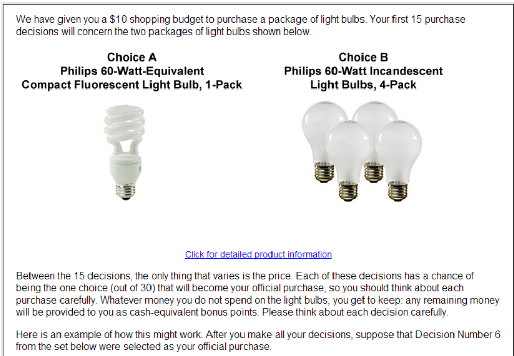
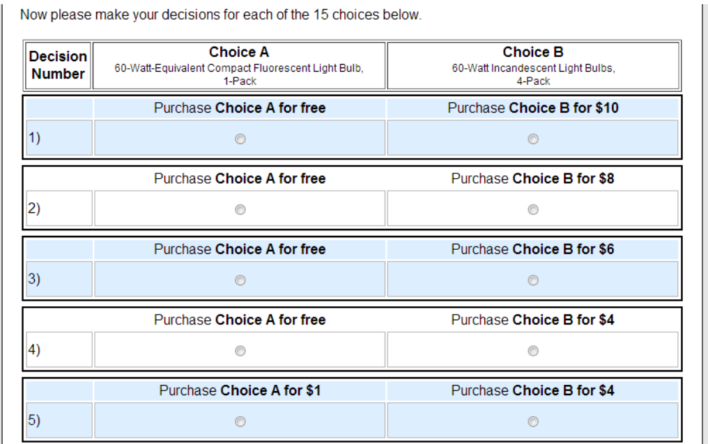
Artefactual field experiment
-
Give consumers $10
-
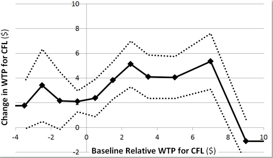
Elicit WTP ($v$) for CFLs
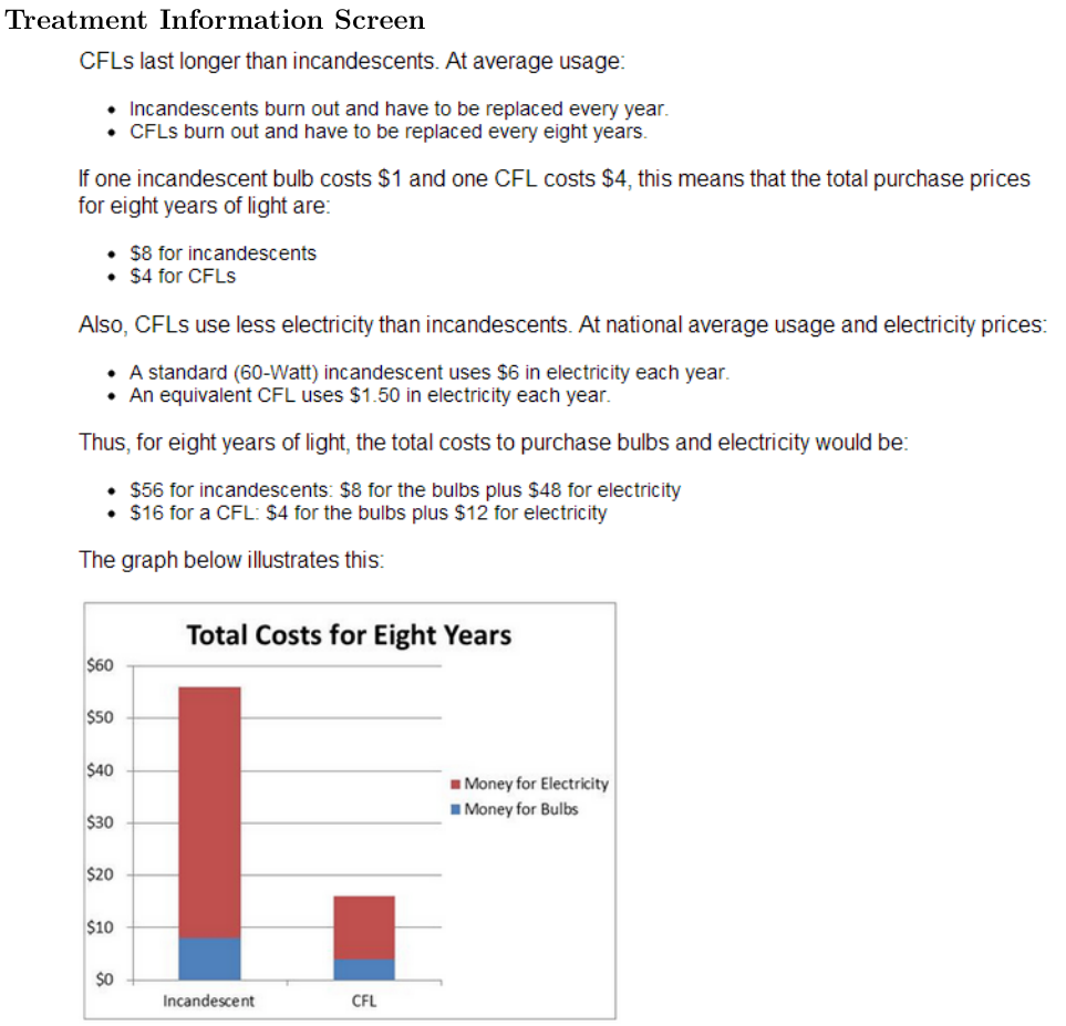
-
Inform some consumers about cost to own to recover $b$
Extend AT model to allow correlation in bias and valuation
-
consumers of type $j$ have distortions $d$ (nests bias from AT)
-
population average $\bar d = \sum \alpha_j d_j$
-
define targeting as:
$$\tau (s) \equiv cov ( d_j, -Q'_j(c-s) )$$
- so a high $\tau(s)$ is well "targetted"
Welfare and optimal subsidy
Result 1:
Poor targeting reduces welfare gains
$$W'(s) = (s - \bar d) \cdot D'(c-s) + \tau(s)$$
Result 2:
Optimal poorly targeted subsidy could be small, even if average bias is large
$$s^* = \bar d - \frac{\tau(s)}{D'(c - s)}$$
[ Optimal subsidy increasing in $\tau(s)$ ]
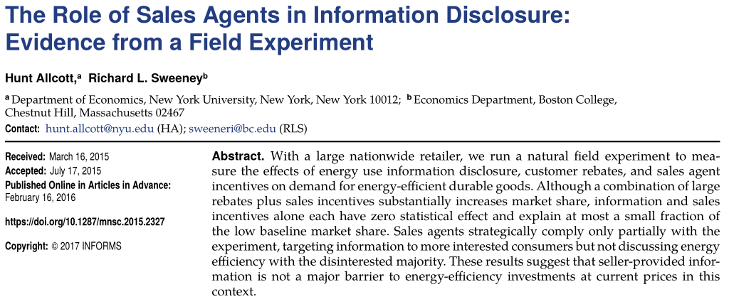
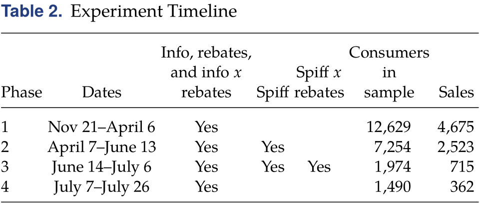
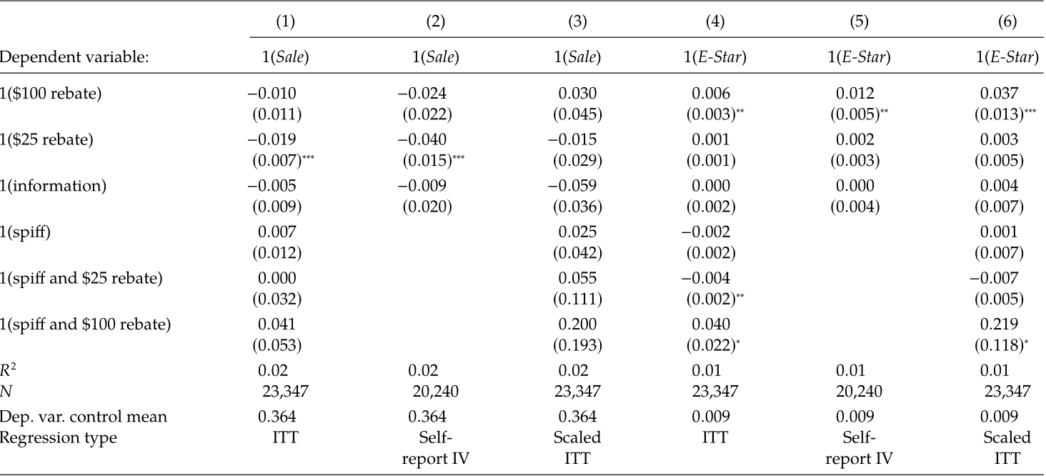
- partner with major appliance retailer
- field experiment at call center
- customer information and rebates
- sales agent incentives
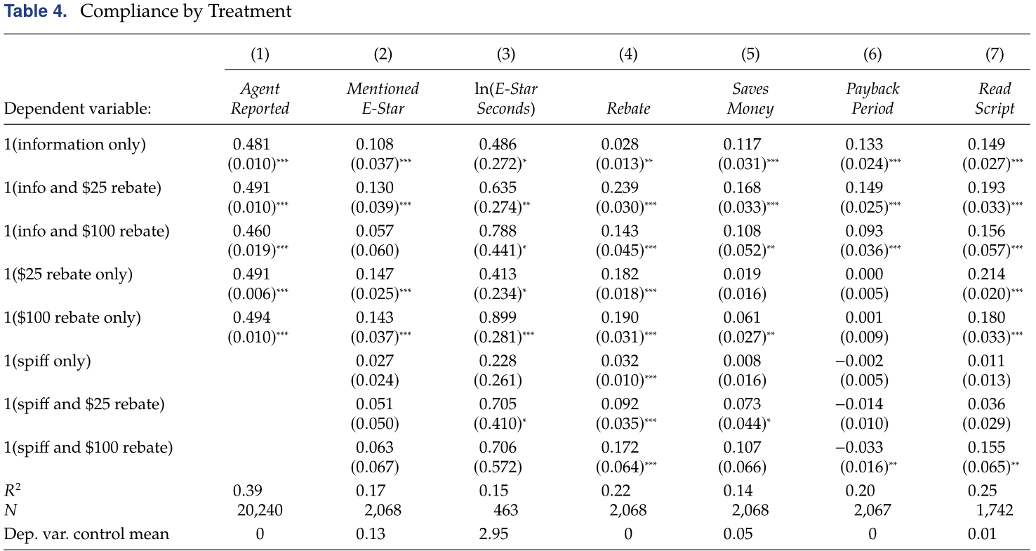
- audit phone calls to check compliance
- survey consumers

Main Results
-
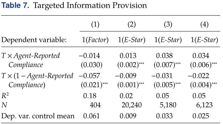
Allcott & Sweeney: Sales agents can target. Can we leverage this somehow?
-
Houde (2014): firms bunch product characteristics around subsidy / label cutoffs
-
Houde (2018): labeling may further reduce average purchased quality